3. Exploratory Data Analysis - Answers

Author

Matthew Ivory

Three important things to remember:

As you complete the handout, please don’t just read the commands, please type every single one of them. This is really important: Learning to program is like practicing a conversation in a new language. You will improve gradually, but only if you practice.
If you’re stuck with something, please write down your questions (to share later in class) and try to solve the problem. Please ask your group members for support and, conversely, if another student is stuck, please try to help them out, too. This way, we develop a supportive learning environment that benefits everybody. In addition, get used to the Help pages in RStudio and start finding solutions online (discussion forums, online textbooks, etc.). This is really important, too. You will only really know how to do quantitative research and statistical analyses when you are doing your own research and dealing with your own data. At that point, you need to be sufficiently autonomous to solve problems, otherwise you will end up making very slow progress in your PhD.
Finally, if you do not complete the handout in class, please complete the handout at home. This is important as we will assume that you know the material covered in this handout. And again, the more you practice the better, so completing these handouts at home is important.

References for this handout

Many of the examples and data files from our class come from these excellent textbooks:

Andrews, M. (2021). Doing data science in R. Sage.
Crawley, M. J. (2013). The R book. Wiley.
Fogarty, B. J. (2019). Quantitative social science data with R. Sage.
Winter, B. (2019). Statistics for linguists. An introduction using R. Routledge.

Step 0: Preparing your Environment

Firt things first, open up a new R script and load in the Tidyverse library

Need a reminder?

library(tidyverse)

In addition, please download the following data files from Moodle (see folder for session 3) and place them in your working directory.

nettle_1999_climate.csv
language_exams_new.csv
scores.csv

Step 1: Tibbles?

In the last session, you have learned how to install the tidyverse package (Wickham, 2017).

tidyverse is a collection of packages that great facilitates data handling in R. In our session on data visualization, you will encounter the ggplot2 package (Wickham, 2016), which is part of tidyverse. Today, we will use functions from other important packages of the tidyverse, namely tibble (Müller & Wickham, 2018), readr (Wickham et al., 2022), and dplyr (Wickham et al., 2018). These are all automatically installed when you install the tidyverse.

We have actually used tibbles last week. When we use the function read_csv(), this reads dataframes and gives them a class of tibble as well as dataframe. We can interpret this as meaning we can apply functions or operations that can apply to both classes.

Tibbles are like the data frames but better. For example, they load much faster, which is important when you are dealing with lots of data.

First, let us load in a tibble/dataframe called languages. The data set comes from Winter’s (2019) textbook.

languages <- read_csv('nettle_1999_climate.csv')

Rows: 74 Columns: 5
── Column specification ────────────────────────────────────────────────────────
Delimiter: ","
chr (1): Country
dbl (4): Population, Area, MGS, Langs

ℹ Use `spec()` to retrieve the full column specification for this data.
ℹ Specify the column types or set `show_col_types = FALSE` to quiet this message.

class(languages)

[1] "spec_tbl_df" "tbl_df"      "tbl"         "data.frame"

What classes are associated with the object languages? Which one means it has been read in as a tibble?

Tip

“tbl” is short for tibble!

Realistically, in future steps/worksheets/discussions, provided we are all on the same page and using read_csv() not read.csv(), then the terms tibble and dataframe are interchangeable.

For completeness sake, and so we can see why working with tibbles is easier, let us read the data again using read.csv(), have a look and compare it against the stored langages object.

For this, let us just read the csv without saving it to an object, you may recall that in week 1, we played about getting R to output various things, we told it to print 2 + 2 and it did just that. It gave us the number 4 in the output. And notice that when we ran languages <- read_csv('nettle_1999_climate.csv') above, we did not get any output. This is because R did what we asked, which was to assign the values of the file to the object called “languages”. Got it? Cool, we can get rid of the left hand side of the assignment operator and just have R read (and print) the values of a file to us. In practice, this is not a useful exercise, but as an educational step, it’s convenient.

Let us run the following command again to have it stored in the environment properly, notice the function is read_csv.

languages <- read_csv('nettle_1999_climate.csv')

Rows: 74 Columns: 5
── Column specification ────────────────────────────────────────────────────────
Delimiter: ","
chr (1): Country
dbl (4): Population, Area, MGS, Langs

ℹ Use `spec()` to retrieve the full column specification for this data.
ℹ Specify the column types or set `show_col_types = FALSE` to quiet this message.

And now:

languages

# A tibble: 74 × 5
   Country      Population  Area   MGS Langs
   <chr>             <dbl> <dbl> <dbl> <dbl>
 1 Algeria            4.41  6.38  6.6     18
 2 Angola             4.01  6.1   6.22    42
 3 Australia          4.24  6.89  6      234
 4 Bangladesh         5.07  5.16  7.4     37
 5 Benin              3.69  5.05  7.14    52
 6 Bolivia            3.88  6.04  6.92    38
 7 Botswana           3.13  5.76  4.6     27
 8 Brazil             5.19  6.93  9.71   209
 9 Burkina Faso       3.97  5.44  5.17    75
10 CAR                3.5   5.79  8.08    94
# ℹ 64 more rows

What’s the difference? As you can see above, the tibble has information about the number of observations (74) and variables (5), the names of the variables: Country, Population, Area, MGS (mean growing season, measured by number of months when crops grow), Langs, and the variable types (character: chr, doubles: dbl, which is a type of numeric vector, and integer: int, also a numeric vector). In addition, the command will display the first ten observations of the variables, lines 1 to 10.

Step 2: Data wrangling

We will now use tidyverse functions for data wrangling. As discussed in our last session, data wrangling is also referred to as data pre-processing or data cleaning. It simply means preparing your raw data (e.g., the data files from experimental software) for statistical analyses. This entails, for example, dealing with missing values, relabeling variables, changing the variable types, etc.

In this part of the handout, we will look at a few tidyverse function that you can use for data wrangling. For more information, I recommend Chapter 3 of Andrews (2021), which provides a comprehensive introduction to data wrangling using tidyverse.

Let’s look at five useful functions for data wrangling with tibbles: filter, select, rename, mutate, and arrange.

Filter

The filter() function can be used, unsurprisingly, to filter rows in your tibble. The filter() function takes the input tibble as its first argument. The second argument is then a logical statement that you can use to filter the data as you please.

Note

We are using pipes, as introduced last week. So here’s some more practice with them coming up. filter() takes the input as the first argument, which means we can pipe the tibble into the filter function.

In the following example, we are reducing the languages tibble to only those rows with countries that have more than 500 languages.

languages |> #pipe object languages
  filter(Langs > 500) # filter rows where variable (column) Langs is greater than 500

# A tibble: 2 × 5
  Country          Population  Area   MGS Langs
  <chr>                 <dbl> <dbl> <dbl> <dbl>
1 Indonesia              5.27  6.28  10.7   701
2 Papua New Guinea       3.58  5.67  10.9   862

Or if you are interested in the data from a specific country (say, Angola), you could simply run the following command. This will only display the rows for Angola.

languages |> 
  filter(Country == "Angola")

# A tibble: 1 × 5
  Country Population  Area   MGS Langs
  <chr>        <dbl> <dbl> <dbl> <dbl>
1 Angola        4.01   6.1  6.22    42

We can even start to get a little bit more adventurous and filter on more than one argument. What about finding countries with more than 500 languages and Population greater than 4?

Warning

Wait! Before running the next line, think about what we are trying to find, look at the previous code we have run in this section, and decide what the expected output should be.

How many rows should be returned? What countries are they going to be?

This kind of mental engagement is critical for your own development - we should also have some kind of mental representation of the information we are getting. It won’t always be super specific, but even just being aware of the shape of a tibble, or general description of the information is important - it means we can check for issues quicker.

languages |> 
  filter(Langs > 500, Population > 4)

# A tibble: 1 × 5
  Country   Population  Area   MGS Langs
  <chr>          <dbl> <dbl> <dbl> <dbl>
1 Indonesia       5.27  6.28  10.7   701

Tip

Indonesia. Look at the output for the code below and notice that it is the same code except we filtered it one step further.

languages |> #pipe object languages
  filter(Langs > 500)

# A tibble: 2 × 5
  Country          Population  Area   MGS Langs
  <chr>                 <dbl> <dbl> <dbl> <dbl>
1 Indonesia              5.27  6.28  10.7   701
2 Papua New Guinea       3.58  5.67  10.9   862

Select

In contrast, you can use the select() function to select specific columns. To do this, simply add the columns you wish to select, separated by commas, as arguments in the function.

languages |> 
  select(Langs, Country)

# A tibble: 74 × 2
   Langs Country     
   <dbl> <chr>       
 1    18 Algeria     
 2    42 Angola      
 3   234 Australia   
 4    37 Bangladesh  
 5    52 Benin       
 6    38 Bolivia     
 7    27 Botswana    
 8   209 Brazil      
 9    75 Burkina Faso
10    94 CAR         
# ℹ 64 more rows

As you might notice, the select() function can also be used to change the sequence of the columns. (In the original tibble, Country came first, followed by Langs.)

On the other hand, if you wish to exclude a column, you can do this by using a minus sign in front of the column in question. The command below will select the four columns Country, Population, Area and MGS, but excluded Langs as requested.

languages |> 
  select(-Langs)

# A tibble: 74 × 4
   Country      Population  Area   MGS
   <chr>             <dbl> <dbl> <dbl>
 1 Algeria            4.41  6.38  6.6 
 2 Angola             4.01  6.1   6.22
 3 Australia          4.24  6.89  6   
 4 Bangladesh         5.07  5.16  7.4 
 5 Benin              3.69  5.05  7.14
 6 Bolivia            3.88  6.04  6.92
 7 Botswana           3.13  5.76  4.6 
 8 Brazil             5.19  6.93  9.71
 9 Burkina Faso       3.97  5.44  5.17
10 CAR                3.5   5.79  8.08
# ℹ 64 more rows

You can also select consecutive columns using :. Let’s take the columns from and including Population, to and including MGS.

languages |> 
  select(Population:MGS)

# A tibble: 74 × 3
   Population  Area   MGS
        <dbl> <dbl> <dbl>
 1       4.41  6.38  6.6 
 2       4.01  6.1   6.22
 3       4.24  6.89  6   
 4       5.07  5.16  7.4 
 5       3.69  5.05  7.14
 6       3.88  6.04  6.92
 7       3.13  5.76  4.6 
 8       5.19  6.93  9.71
 9       3.97  5.44  5.17
10       3.5   5.79  8.08
# ℹ 64 more rows

It is worth noting that getting filter() and select() mixed up is pretty common. I personally do it a lot. A vaguely helpful way to remember is that filteR is for Rows and select is not. Or seleCt is for Columns? Or jsut do what I do, and get it wrong 50% of the time, and then just change it when you get the error!

Rename

A third useful function is called rename(). This function can be used to change the name of columns. To do this, you first write the new column (here, Population) followed by an equal sign (=) and the old column name (Pop).

rename() is useful for when we have really messy taking that comes from an online survey, government statistics, or even a PsychoPy study. We could tidy data in excel before reading into R, but that defeats the point of using R and being a successful data scientist (which is you!) - it reduces the reproduciblity and transparency of your analyses from start to finish.

languages <- languages |> #here we are manipulating in place the object languages. We are overwriting the existing object
  rename(Pop = Population)

Warning

Woah, woah, woah - what did I just do to the object languages? I assigned the object languages to languages? Not quite. I assigned the entire of the right hand side of the assignment operator to overwrite the same object. So I renamed a column and saved it to the existing object. Analogy: like saving over the top of a word document. Or, to see a basic example in action, make sure you have the environment pane selected in the top right and run the next command, see what shows, and then run the second and see what changed. It should be pretty clear what will happen, but just extrapolate that to tibbles and renaming (we could have also reassigned any of the previous actions we took using filter or select).

x <- 32

x <- 64

Mutate

The mutate() function can be used to change the content of a tibble. For example, you can add an additional column, which in the example below will be the Langs column divided by 100.

languages <- languages |> 
  mutate(Langs100 = Langs/100)

head(languages) # show me the top 6 rows

# A tibble: 6 × 6
  Country      Pop  Area   MGS Langs Langs100
  <chr>      <dbl> <dbl> <dbl> <dbl>    <dbl>
1 Algeria     4.41  6.38  6.6     18     0.18
2 Angola      4.01  6.1   6.22    42     0.42
3 Australia   4.24  6.89  6      234     2.34
4 Bangladesh  5.07  5.16  7.4     37     0.37
5 Benin       3.69  5.05  7.14    52     0.52
6 Bolivia     3.88  6.04  6.92    38     0.38

We can also use mutate() to change specific values to something else. Look at this example dataset:

#let's create a 2x3 tibble with two participants, who both took part in a study where we tested their working memory, and one was in the control group (1 for yes, 0 for no) and the other was not
test_data <- tibble(name = c("Jenny", "Jonny"), 
                    score = c(45, 23),
                    control_group = c(1,0))

test_data

# A tibble: 2 × 3
  name  score control_group
  <chr> <dbl>         <dbl>
1 Jenny    45             1
2 Jonny    23             0

Looking at the variable control_group it may not be clear to everyone what 1 or 0 means, so let’s use mutate() to update this variable

test_data_update <- test_data |> 
  mutate(control_group = str_replace(control_group, "1",  "yes"),
         control_group = str_replace(control_group, "0",  "no"))

Looks pretty complicated! Let’s break it down:

The first line tells us what the new object will be, and what data we are starting with, we are then piping that into:
mutate() which then tells us we want to update the control_group variable. and we want to apply a new function called str_replace which replaces strings. We are saying “look in the variable control group, and if we find a ‘1’, replace it with the string ‘yes’. We end the second line with a comma telling R we are doing something more
line three then repeats line two (still inside mutate if you follow the parentheses), and looks for a ‘0’ and replaces it with ‘no’. And we finish there.

Check out both obhjects, what’s changed?

test_data

# A tibble: 2 × 3
  name  score control_group
  <chr> <dbl>         <dbl>
1 Jenny    45             1
2 Jonny    23             0

test_data_update

# A tibble: 2 × 3
  name  score control_group
  <chr> <dbl> <chr>        
1 Jenny    45 yes          
2 Jonny    23 no

The arguments in str_replace() want three things: the column it is checking, the strong it is looking for, and the string to replace it with. What if we wanted 1 to equal “control” and 0 to equal “experiment” instead? Try it out.

We will explore mutate() more in later weeks, but know that it is a very useful and powerful tool. It will be a common tool in your data science belt. It can be used in conjunction with other functions to do some really cool things. As a quick teaser, what if we wanted to know the population density per area unit?

languages <- languages |> 
  mutate(density = Pop/Area) #We divide the total population by the area

If you took the time to calculate each row, you will see that for every row mutate() has taken the specific value of Pop and divided it by Area. Neat, that will save us a lot of time! Just know that we can make these even more complex…

Arrange

Finally, the arrange() function can be used to order a tibble in ascending or descending order. In the example below, we are use this function to first look at the countries with the smallest number of languages (Cuba, Madagascar, etc.), followed by the countries with the largest numbers of languages (Papua New Guinea, Indonesia, Nigeria, etc.).

languages |> 
  arrange(Langs)

# A tibble: 74 × 7
   Country        Pop  Area   MGS Langs Langs100 density
   <chr>        <dbl> <dbl> <dbl> <dbl>    <dbl>   <dbl>
 1 Cuba          4.03  5.04  7.46     1     0.01   0.800
 2 Madagascar    4.06  5.77  7.33     4     0.04   0.704
 3 Yemen         4.09  5.72  0        6     0.06   0.715
 4 Nicaragua     3.6   5.11  8.13     7     0.07   0.705
 5 Sri Lanka     4.24  4.82  9.59     7     0.07   0.880
 6 Mauritania    3.31  6.01  0.75     8     0.08   0.551
 7 Oman          3.19  5.33  0        8     0.08   0.598
 8 Saudi Arabia  4.17  6.33  0.4      8     0.08   0.659
 9 Honduras      3.72  5.05  8.54     9     0.09   0.737
10 UAE           3.21  4.92  0.83     9     0.09   0.652
# ℹ 64 more rows

or in descending order?

languages |> 
  arrange(desc(Langs))

# A tibble: 74 × 7
   Country            Pop  Area   MGS Langs Langs100 density
   <chr>            <dbl> <dbl> <dbl> <dbl>    <dbl>   <dbl>
 1 Papua New Guinea  3.58  5.67 10.9    862     8.62   0.631
 2 Indonesia         5.27  6.28 10.7    701     7.01   0.839
 3 Nigeria           5.05  5.97  7      427     4.27   0.846
 4 India             5.93  6.52  5.32   405     4.05   0.910
 5 Cameroon          4.09  5.68  9.17   275     2.75   0.720
 6 Mexico            4.94  6.29  5.84   243     2.43   0.785
 7 Australia         4.24  6.89  6      234     2.34   0.615
 8 Zaire             4.56  6.37  9.44   219     2.19   0.716
 9 Brazil            5.19  6.93  9.71   209     2.09   0.749
10 Philippines       4.8   5.48 10.3    168     1.68   0.876
# ℹ 64 more rows

#which is functionally equivalent to:
#
#languages |> 
# arrange(-Langs)

Before we move on, let’s clean up our environment and we are wanting to start with a fresh one for the rest of the worksheet.

We can use the function rm() to remove items from the environment pane. We should have two items, x and languages.

rm(x)
rm(languages)

Step 3: Exploratory Data Analysis

We are now ready for some exploratory data analysis in R. First, let’s load the three data files as tibbles. To load the data sets as tibbles, we use the read_csv() function

Rows: 74 Columns: 5
── Column specification ────────────────────────────────────────────────────────
Delimiter: ","
chr (1): Country
dbl (4): Population, Area, MGS, Langs

ℹ Use `spec()` to retrieve the full column specification for this data.
ℹ Specify the column types or set `show_col_types = FALSE` to quiet this message.
Rows: 1000 Columns: 5
── Column specification ────────────────────────────────────────────────────────
Delimiter: ","
dbl (5): student_id, age, exam_1, exam_2, exam_3

ℹ Use `spec()` to retrieve the full column specification for this data.
ℹ Specify the column types or set `show_col_types = FALSE` to quiet this message.
Rows: 21 Columns: 1
── Column specification ────────────────────────────────────────────────────────
Delimiter: ","
dbl (1): scores

ℹ Use `spec()` to retrieve the full column specification for this data.
ℹ Specify the column types or set `show_col_types = FALSE` to quiet this message.

Once you have loaded the data sets and created the new tibbles, it’s good to inspect the data to make sure all was imported properly. This is important before you do any analyses. Remember: “Garbage in, garbage out.”

You can use the View(), head(), and str() functions. Personally I suggest using head() to get a first idea.

We are now ready to calculate a few summary statistics! We did some of this in prior worksheets, but we will see some more here.

Mean

To calculate the arithmetic mean, you can use the mean() function.

mean(test_scores$scores)

[1] 612.2381

In the case of language_exams_new, we have three exams for which we might want to know the mean.

mean(language_exams_new$exam_1)

[1] 68.052

mean(language_exams_new$exam_2)

[1] 75.055

mean(language_exams_new$exam_3)

[1] 87.918

But rather than calculating the mean for each column separately (exam_1 to exam_3), we can use the colMeans() function to calculate the mean for all columns.

colMeans(language_exams_new)

student_id        age     exam_1     exam_2     exam_3 
 16326.612     24.705     68.052     75.055     87.918

Note that for student_id the output is essentially meaningless; it might be worth to filter out this variable (well, unselect the column. We could do this using two pipes:

language_exams_new |> # take the object language_exams_new
  select(-student_id) |> # deselect the column student_id
  colMeans() # apply the function colMeans()

   age exam_1 exam_2 exam_3 
24.705 68.052 75.055 87.918

If the above looks really complicated, it isn’t - don’t worry! Let us break it down. Look at the first two lines of code: we take the object language_exams_new and pipe it into the select function and remove the column student_id. We’ve done this before, this isn’t new. We are then seeing another pipe! This means that everything on the LHS of that pipe is shifted into the first spot of the RHS, so we are taken the object minus student_id and applying col_means(). That wasn’t so bad, it’s quite clear when we think about it programmatically.

Consider that we can take this same approach and keep adding pipes for ever and ever, always doing the same thing: evaluate the first line and the bit between two pipes, then all of the LHS goes through the next pipe into the next function, and then so on, ever building in its pipeline, creating something complex at the end. That’s enough of this for now, we can get more practice later on, but it will help you to structure and read complicated code and make you into the great data scientist that you are.

Trimmed Mean

The trimmed mean is useful when we want to exclude extreme values. Remember though that any data exclusion needs to be justified and it needs to be described in your report. There is a significant degree of trust that you report everything that you carried out in your analysis transparently.

Compare the two outputs, with and without the extreme values. The trim argument here deletes the bottom and top 10% of scores.

mean(test_scores$scores)

[1] 612.2381

mean(test_scores$scores, trim = 0.1)

[1] 508.5882

Median

The median is calculated by using the following command.

median(test_scores$scores)

[1] 465

median (language_exams_new$exam_1)

[1] 68

Standard Deviation

sd(test_scores$scores)

[1] 552.2874

sd(language_exams_new$exam_1)

[1] 2.049755

Range

The range can provide useful information about our sample data. For example, let’s calculate the age range of participants in language_exams_new.

The range() function does not give you the actual range. It only provides the minimum and maximum values.

range(language_exams_new$age)

[1] 17 38

To calculate the range, we can ask R to give us the different between the two values reported by range

range(language_exams_new$age) |> 
  diff()

[1] 21

diff() is a new function, and one we probably won’t use too much more, so it doesn’t deserve much space, diff is short for difference, so it calculates the difference between two values. That’s all really, but look how we take one output that wasn’t useful by itself and applied a new function to get something useful!

Note

If you want to know a (not-so) fun fact, before writing this worksheet, I didn’t even know that diff() existed. I guessed it would (which is based off experience, so not helpful for you to know), but I then checked it did what I thought it did by running ?diff (in the console, NOT script) and it confirmed my suspicions. I could also have just googled “R difference between two values” and read the top two results.

Quantiles

Quantiles can easily be displayed by means of the quantile() function, as you can see in the example below.

quantile(language_exams_new$exam_1)

  0%  25%  50%  75% 100% 
  62   67   68   69   74

In our exam_1 data, each of the quantiles above tells us how many scores are below the given the value. For example, 0% of scores are below 62, meaning that 62 is the lowest score. 50% of scores are below 68 and 50% above 68. (The 50% quantile is the median.) And 100% of scores are below 74, meaning that 74 is the highest score in the data set.

We can confirm that this is true by using the range() function, which confirms 62 and 74 as minimum and maximum values. Can you remember (or look back) to see how we would do this?

[1] 62 74

Sometimes, we want to calculate a specific one, e.g. a percentile. For this, you can add the following arguments to the quantile() function. For example, to display the 10% and 90% quantiles, you would add 0.1 and 0.9 respectively, as in the examples below.

quantile(language_exams_new$exam_1, 0.1)

10% 
 65

quantile(language_exams_new$exam_1, 0.9)

90% 
 71

Summary

The summary() function is a fast way to get the key summary statistics.

summary(language_exams_new)

   student_id         age           exam_1          exam_2          exam_3     
 Min.   :10011   Min.   :17.0   Min.   :62.00   Min.   :70.00   Min.   :81.00  
 1st Qu.:13028   1st Qu.:20.0   1st Qu.:67.00   1st Qu.:74.00   1st Qu.:87.00  
 Median :15988   Median :23.0   Median :68.00   Median :75.00   Median :88.00  
 Mean   :16327   Mean   :24.7   Mean   :68.05   Mean   :75.06   Mean   :87.92  
 3rd Qu.:19070   3rd Qu.:28.0   3rd Qu.:69.00   3rd Qu.:76.00   3rd Qu.:89.00  
 Max.   :24996   Max.   :38.0   Max.   :74.00   Max.   :81.00   Max.   :97.00

summary() is actually quite messy, but it is quick and sometimes that’s all we need, just to get a rough idea of the shape of the data.

Frequencies

Sometimes it is helpful to observe the frequencies in our sample data. The freq() function is really helpful for this. Note: This function requires the descr package, which we will need to install and then load. Can you remember where we put these two respective commands? One goes in the console, and one at the top of the script.

install.packages("descr")

library(descr)

library(descr)

Warning: package 'descr' was built under R version 4.2.3

Note

install.packages("descr") #in the console because it is temporary

library(descr) #at the top of the script because we need it to show everyone what tools they need

The following command will create a frequency table. On the left, you will see the score, in the middle the frequency with which the score occurs, and to the right this is express in percentage points. This tells you, for example, that the most frequent score (the mode) is 68, the least frequent score is 62.

freq(language_exams_new$exam_1, plot = FALSE)

language_exams_new$exam_1 
      Frequency Percent
62            2     0.2
63           13     1.3
64           27     2.7
65           68     6.8
66          109    10.9
67          168    16.8
68          196    19.6
69          175    17.5
70          139    13.9
71           56     5.6
72           32     3.2
73           12     1.2
74            3     0.3
Total      1000   100.0

Frequencies with a twist

If you omit the argument plot = FALSE in the freq() function (which just default the argument plot = TRUE, check it out in the help pane and searching for the function name), R will produce both a table and a visual display of your data. Compare the table and the histogram (the graph). Which one is more informative? What are the relative advantages of either?

freq(language_exams_new$exam_1)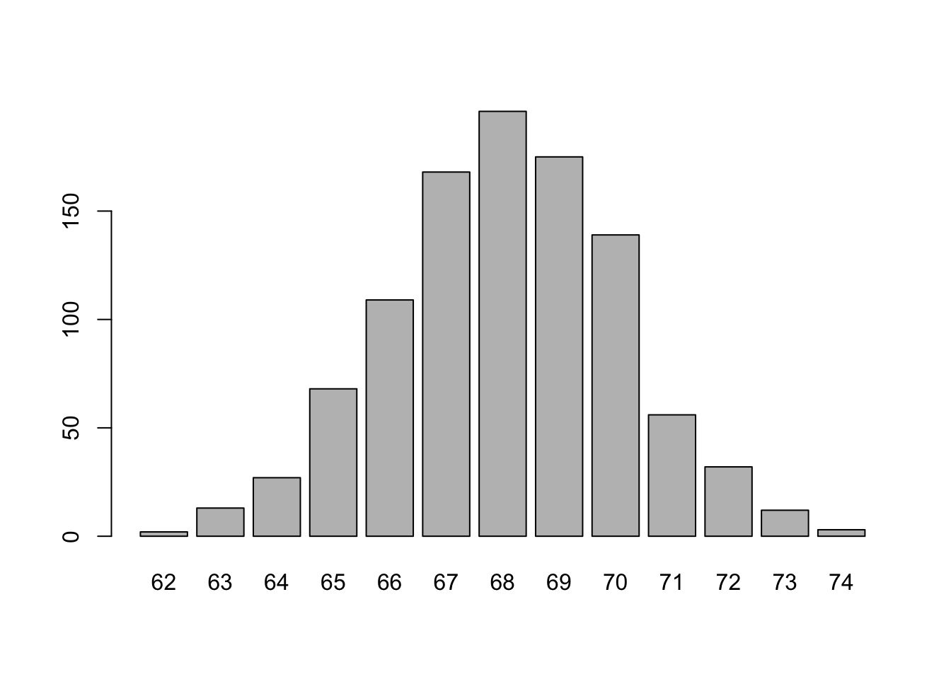

language_exams_new$exam_1 
      Frequency Percent
62            2     0.2
63           13     1.3
64           27     2.7
65           68     6.8
66          109    10.9
67          168    16.8
68          196    19.6
69          175    17.5
70          139    13.9
71           56     5.6
72           32     3.2
73           12     1.2
74            3     0.3
Total      1000   100.0

For now, we can keep the colour grey. Next week we can play with colours properly, but for now - just know you can make some great plots, but for basic exploration, let’s keep them fast and basic because we just need to know the basic shape of the data

Step 4: Our first graphic explorations

To conclude, let’s try out a few basic graphics. Next week, we will go into much more detail, but here’s a preview of data visualization. The graphics below are available in the R base package. By and large, this will be your only exposure to base plots, because they aren’t as useful or smart as tidy plots, but for fast visualisation, they’re “just ok”. Don’t get too attached to them, next week we get some real exposure to graphics.

Boxplot

Boxplots are helpful to inspect the data (Tukey, 1977), as discussed in our lecture today. The following command creates a boxplot, based on exam_1 from the data set language_exams_new.

boxplot(language_exams_new$exam_1)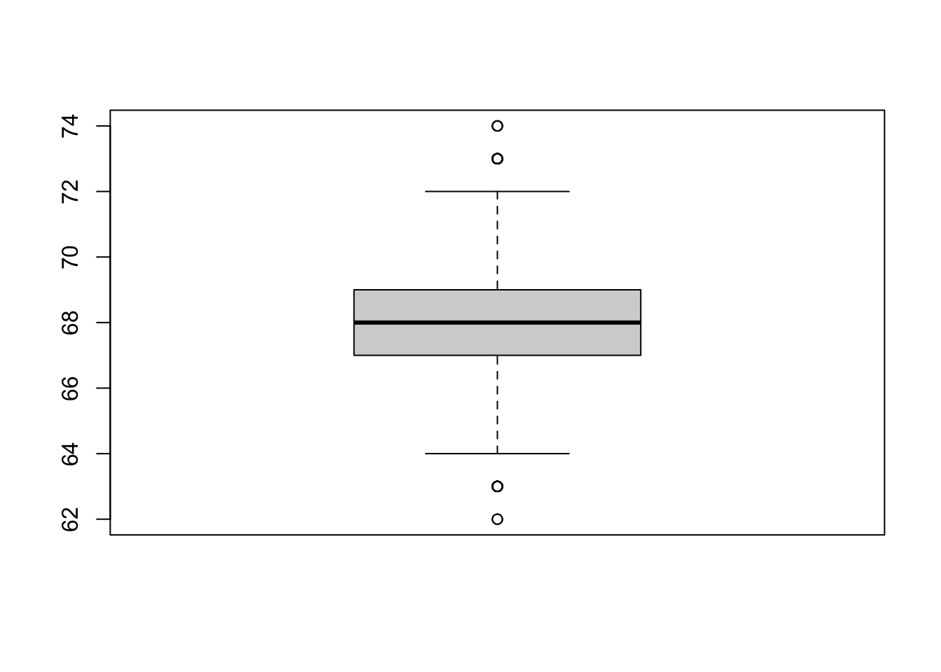

What if we want to compare performance on all three exams (exam_1, exam_2, exam_3) next to each other?

One way of doing this (there are other ways) is to first create three new objects exam_1, exam_2, exam_3, and then used the boxplot() function on the three.

Have a go.

exam_1 <- c(language_exams_new$exam_1) 

exam_2 <- c(language_exams_new$exam_2) 

exam_3 <- c(language_exams_new$exam_3) 

boxplot(exam_1, exam_2, exam_3)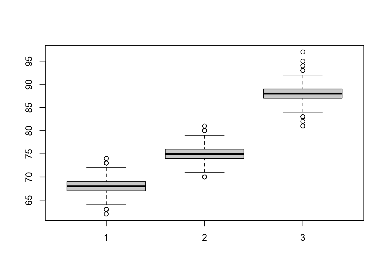

Could you run the above using just one line? What is easier to read? What do you prefer?

Histograms

Last but not least, histograms are helpful ways to visually inspect your data. To create a histogram, simply use the hist() function, as in the following examples.

hist(language_exams_new$exam_3)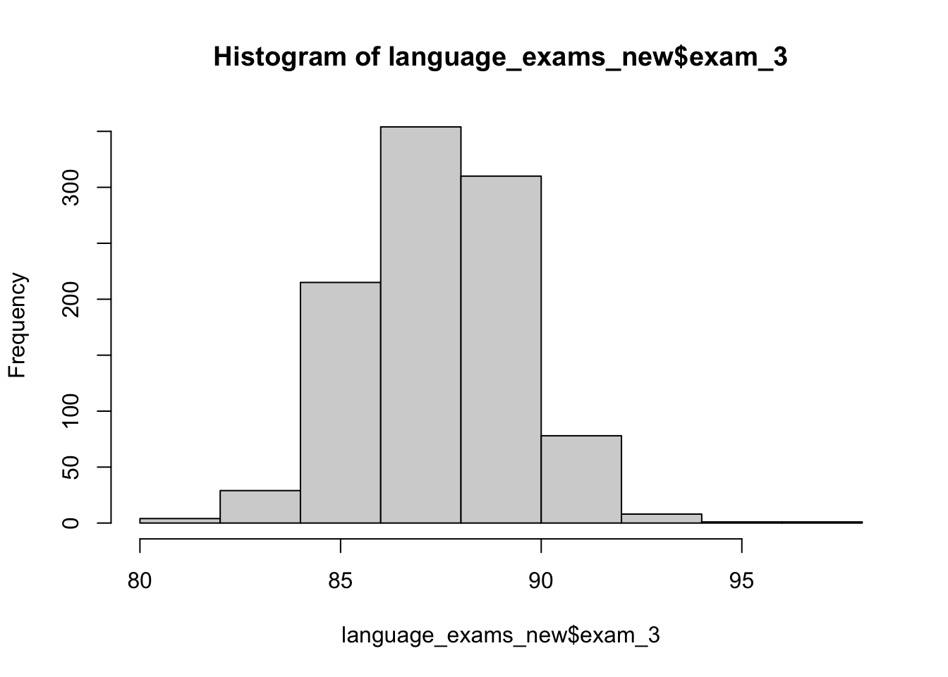

Take home task

None this week. You’ve worked hard and learnt a lot of complicated aspects of R - your task can be relish in your new found knowledge and be impressed with what you can now do in R.

Next week we take on graphs, plots, and visualisations!